Challenge 8

challenge_8
faostat
Joining Data
Author

Mekhala Kumar

Published

August 25, 2022

library(tidyverse)
library(ggplot2)
library(readr)

knitr::opts_chunk$set(echo = TRUE, warning=FALSE, message=FALSE)

Description of the data

Two datasets have been used for this dataset- the FAOSTAT cattle and the FAOSTAT chicken ones. They are time-series datasets with information about the amount of eggs and chicken yielded or produced. The information is present for several countries.

dairy <- read_csv("_data/FAOSTAT_cattle_dairy.csv")
egg <- read_csv("_data/FAOSTAT_egg_chicken.csv")
dim(dairy)
[1] 36449    14
dim(egg)
[1] 38170    14
print(summarytools::dfSummary(dairy,
                        varnumbers = FALSE,
                        plain.ascii  = FALSE, 
                        style        = "grid", 
                        graph.magnif = 0.70, 
                        valid.col    = FALSE),
      method = 'render',
      table.classes = 'table-condensed')

Data Frame Summary

dairy

Dimensions: 36449 x 14
Duplicates: 0
Variable Stats / Values Freqs (% of Valid) Graph Missing
Domain Code [character] 1. QL
36449(100.0%)
0 (0.0%)
Domain [character] 1. Livestock Primary
36449(100.0%)
0 (0.0%)
Area Code [numeric]
Mean (sd) : 775.2 (1713.8)
min ≤ med ≤ max:
1 ≤ 141 ≤ 5504
IQR (CV) : 146 (2.2)
232 distinct values 0 (0.0%)
Area [character]
1. Afghanistan
2. Africa
3. Albania
4. Algeria
5. American Samoa
6. Americas
7. Angola
8. Antigua and Barbuda
9. Argentina
10. Asia
[ 222 others ]
174(0.5%)
174(0.5%)
174(0.5%)
174(0.5%)
174(0.5%)
174(0.5%)
174(0.5%)
174(0.5%)
174(0.5%)
174(0.5%)
34709(95.2%)
0 (0.0%)
Element Code [numeric]
Mean (sd) : 5416 (78.5)
min ≤ med ≤ max:
5318 ≤ 5420 ≤ 5510
IQR (CV) : 192 (0)
5318:12158(33.4%)
5420:12121(33.3%)
5510:12170(33.4%)
0 (0.0%)
Element [character]
1. Milk Animals
2. Production
3. Yield
12158(33.4%)
12170(33.4%)
12121(33.3%)
0 (0.0%)
Item Code [numeric] 1 distinct value
882:36449(100.0%)
0 (0.0%)
Item [character] 1. Milk, whole fresh cow
36449(100.0%)
0 (0.0%)
Year Code [numeric]
Mean (sd) : 1990.4 (16.8)
min ≤ med ≤ max:
1961 ≤ 1991 ≤ 2018
IQR (CV) : 29 (0)
58 distinct values 0 (0.0%)
Year [numeric]
Mean (sd) : 1990.4 (16.8)
min ≤ med ≤ max:
1961 ≤ 1991 ≤ 2018
IQR (CV) : 29 (0)
58 distinct values 0 (0.0%)
Unit [character]
1. Head
2. hg/An
3. tonnes
12158(33.4%)
12121(33.3%)
12170(33.4%)
0 (0.0%)
Value [numeric]
Mean (sd) : 4410235 (25744621)
min ≤ med ≤ max:
7 ≤ 43266 ≤ 683217055
IQR (CV) : 692151 (5.8)
24088 distinct values 74 (0.2%)
Flag [character]
1. *
2. A
3. F
4. Fc
5. Im
6. M
810(3.1%)
3070(11.6%)
7045(26.7%)
13136(49.7%)
2270(8.6%)
74(0.3%)
10044 (27.6%)
Flag Description [character]
1. Aggregate, may include of
2. Calculated data
3. Data not available
4. FAO data based on imputat
5. FAO estimate
6. Official data
7. Unofficial figure
3070(8.4%)
13136(36.0%)
74(0.2%)
2270(6.2%)
7045(19.3%)
10044(27.6%)
810(2.2%)
0 (0.0%)

Generated by summarytools 1.0.1 (R version 4.2.1)
2022-08-25

print(summarytools::dfSummary(egg,
                        varnumbers = FALSE,
                        plain.ascii  = FALSE, 
                        style        = "grid", 
                        graph.magnif = 0.70, 
                        valid.col    = FALSE),
      method = 'render',
      table.classes = 'table-condensed')

Data Frame Summary

egg

Dimensions: 38170 x 14
Duplicates: 0
Variable Stats / Values Freqs (% of Valid) Graph Missing
Domain Code [character] 1. QL
38170(100.0%)
0 (0.0%)
Domain [character] 1. Livestock Primary
38170(100.0%)
0 (0.0%)
Area Code [numeric]
Mean (sd) : 771.1 (1709.6)
min ≤ med ≤ max:
1 ≤ 143 ≤ 5504
IQR (CV) : 145 (2.2)
245 distinct values 0 (0.0%)
Area [character]
1. Afghanistan
2. Africa
3. Albania
4. Algeria
5. American Samoa
6. Americas
7. Angola
8. Antigua and Barbuda
9. Argentina
10. Asia
[ 235 others ]
174(0.5%)
174(0.5%)
174(0.5%)
174(0.5%)
174(0.5%)
174(0.5%)
174(0.5%)
174(0.5%)
174(0.5%)
174(0.5%)
36430(95.4%)
0 (0.0%)
Element Code [numeric]
Mean (sd) : 5411.4 (80.5)
min ≤ med ≤ max:
5313 ≤ 5410 ≤ 5510
IQR (CV) : 197 (0)
5313:12679(33.2%)
5410:12651(33.1%)
5510:12840(33.6%)
0 (0.0%)
Element [character]
1. Laying
2. Production
3. Yield
12679(33.2%)
12840(33.6%)
12651(33.1%)
0 (0.0%)
Item Code [numeric] 1 distinct value
1062:38170(100.0%)
0 (0.0%)
Item [character] 1. Eggs, hen, in shell
38170(100.0%)
0 (0.0%)
Year Code [numeric]
Mean (sd) : 1990.5 (16.7)
min ≤ med ≤ max:
1961 ≤ 1991 ≤ 2018
IQR (CV) : 29 (0)
58 distinct values 0 (0.0%)
Year [numeric]
Mean (sd) : 1990.5 (16.7)
min ≤ med ≤ max:
1961 ≤ 1991 ≤ 2018
IQR (CV) : 29 (0)
58 distinct values 0 (0.0%)
Unit [character]
1. 1000 Head
2. 100mg/An
3. tonnes
12679(33.2%)
12651(33.1%)
12840(33.6%)
0 (0.0%)
Value [numeric]
Mean (sd) : 291341.2 (2232761)
min ≤ med ≤ max:
1 ≤ 31996 ≤ 76769955
IQR (CV) : 91235.8 (7.7)
21325 distinct values 40 (0.1%)
Flag [character]
1. *
2. A
3. F
4. Fc
5. Im
6. M
1435(4.7%)
3186(10.4%)
10538(34.4%)
13344(43.6%)
2079(6.8%)
40(0.1%)
7548 (19.8%)
Flag Description [character]
1. Aggregate, may include of
2. Calculated data
3. Data not available
4. FAO data based on imputat
5. FAO estimate
6. Official data
7. Unofficial figure
3186(8.3%)
13344(35.0%)
40(0.1%)
2079(5.4%)
10538(27.6%)
7548(19.8%)
1435(3.8%)
0 (0.0%)

Generated by summarytools 1.0.1 (R version 4.2.1)
2022-08-25

Tidy Data (as needed)

The data is already tidy in both the datasets. In the item column, there was unnecessary text so I removed that.

dairy<-dairy%>%mutate(Item=str_remove(Item,", whole fresh cow"))
egg<-egg%>%mutate(Item=str_remove(Item,", hen, in shell"))

Join Data

At first, I joined the datasets by doing an inner join and using the common column as year. However, both the datasets, have the same column names and information and using inner join created more columns, essentially a duplicate, with the same information.
I realised that I wanted to add the rows from the FAOSTAT chicken dataset to the existing FAOSTAT cattle dataset. Therefore, I used rbind() to join the two datasets.

#full_join()
dairy_egg<-dairy %>% 
  inner_join(egg, by = "Year")

head(dairy_egg)
# A tibble: 6 × 27
  Domain C…¹ Domai…² Area …³ Area.x Eleme…⁴ Eleme…⁵ Item …⁶ Item.x Year …⁷  Year
  <chr>      <chr>     <dbl> <chr>    <dbl> <chr>     <dbl> <chr>    <dbl> <dbl>
1 QL         Livest…       2 Afgha…    5318 Milk A…     882 Milk      1961  1961
2 QL         Livest…       2 Afgha…    5318 Milk A…     882 Milk      1961  1961
3 QL         Livest…       2 Afgha…    5318 Milk A…     882 Milk      1961  1961
4 QL         Livest…       2 Afgha…    5318 Milk A…     882 Milk      1961  1961
5 QL         Livest…       2 Afgha…    5318 Milk A…     882 Milk      1961  1961
6 QL         Livest…       2 Afgha…    5318 Milk A…     882 Milk      1961  1961
# … with 17 more variables: Unit.x <chr>, Value.x <dbl>, Flag.x <chr>,
#   `Flag Description.x` <chr>, `Domain Code.y` <chr>, Domain.y <chr>,
#   `Area Code.y` <dbl>, Area.y <chr>, `Element Code.y` <dbl>, Element.y <chr>,
#   `Item Code.y` <dbl>, Item.y <chr>, `Year Code.y` <dbl>, Unit.y <chr>,
#   Value.y <dbl>, Flag.y <chr>, `Flag Description.y` <chr>, and abbreviated
#   variable names ¹​`Domain Code.x`, ²​Domain.x, ³​`Area Code.x`,
#   ⁴​`Element Code.x`, ⁵​Element.x, ⁶​`Item Code.x`, ⁷​`Year Code.x`
# ℹ Use `colnames()` to see all variable names
tail(dairy_egg)
# A tibble: 6 × 27
  Domain C…¹ Domai…² Area …³ Area.x Eleme…⁴ Eleme…⁵ Item …⁶ Item.x Year …⁷  Year
  <chr>      <chr>     <dbl> <chr>    <dbl> <chr>     <dbl> <chr>    <dbl> <dbl>
1 QL         Livest…    5504 Polyn…    5510 Produc…     882 Milk      2018  2018
2 QL         Livest…    5504 Polyn…    5510 Produc…     882 Milk      2018  2018
3 QL         Livest…    5504 Polyn…    5510 Produc…     882 Milk      2018  2018
4 QL         Livest…    5504 Polyn…    5510 Produc…     882 Milk      2018  2018
5 QL         Livest…    5504 Polyn…    5510 Produc…     882 Milk      2018  2018
6 QL         Livest…    5504 Polyn…    5510 Produc…     882 Milk      2018  2018
# … with 17 more variables: Unit.x <chr>, Value.x <dbl>, Flag.x <chr>,
#   `Flag Description.x` <chr>, `Domain Code.y` <chr>, Domain.y <chr>,
#   `Area Code.y` <dbl>, Area.y <chr>, `Element Code.y` <dbl>, Element.y <chr>,
#   `Item Code.y` <dbl>, Item.y <chr>, `Year Code.y` <dbl>, Unit.y <chr>,
#   Value.y <dbl>, Flag.y <chr>, `Flag Description.y` <chr>, and abbreviated
#   variable names ¹​`Domain Code.x`, ²​Domain.x, ³​`Area Code.x`,
#   ⁴​`Element Code.x`, ⁵​Element.x, ⁶​`Item Code.x`, ⁷​`Year Code.x`
# ℹ Use `colnames()` to see all variable names
dim(dairy_egg)
[1] 24076265       27
new_dairy_egg<-rbind(dairy,egg)
head(new_dairy_egg)
# A tibble: 6 × 14
  Domai…¹ Domain Area …² Area  Eleme…³ Element Item …⁴ Item  Year …⁵  Year Unit 
  <chr>   <chr>    <dbl> <chr>   <dbl> <chr>     <dbl> <chr>   <dbl> <dbl> <chr>
1 QL      Lives…       2 Afgh…    5318 Milk A…     882 Milk     1961  1961 Head 
2 QL      Lives…       2 Afgh…    5420 Yield       882 Milk     1961  1961 hg/An
3 QL      Lives…       2 Afgh…    5510 Produc…     882 Milk     1961  1961 tonn…
4 QL      Lives…       2 Afgh…    5318 Milk A…     882 Milk     1962  1962 Head 
5 QL      Lives…       2 Afgh…    5420 Yield       882 Milk     1962  1962 hg/An
6 QL      Lives…       2 Afgh…    5510 Produc…     882 Milk     1962  1962 tonn…
# … with 3 more variables: Value <dbl>, Flag <chr>, `Flag Description` <chr>,
#   and abbreviated variable names ¹​`Domain Code`, ²​`Area Code`,
#   ³​`Element Code`, ⁴​`Item Code`, ⁵​`Year Code`
# ℹ Use `colnames()` to see all variable names
tail(new_dairy_egg)
# A tibble: 6 × 14
  Domai…¹ Domain Area …² Area  Eleme…³ Element Item …⁴ Item  Year …⁵  Year Unit 
  <chr>   <chr>    <dbl> <chr>   <dbl> <chr>     <dbl> <chr>   <dbl> <dbl> <chr>
1 QL      Lives…    5504 Poly…    5313 Laying     1062 Eggs     2017  2017 1000…
2 QL      Lives…    5504 Poly…    5410 Yield      1062 Eggs     2017  2017 100m…
3 QL      Lives…    5504 Poly…    5510 Produc…    1062 Eggs     2017  2017 tonn…
4 QL      Lives…    5504 Poly…    5313 Laying     1062 Eggs     2018  2018 1000…
5 QL      Lives…    5504 Poly…    5410 Yield      1062 Eggs     2018  2018 100m…
6 QL      Lives…    5504 Poly…    5510 Produc…    1062 Eggs     2018  2018 tonn…
# … with 3 more variables: Value <dbl>, Flag <chr>, `Flag Description` <chr>,
#   and abbreviated variable names ¹​`Domain Code`, ²​`Area Code`,
#   ³​`Element Code`, ⁴​`Item Code`, ⁵​`Year Code`
# ℹ Use `colnames()` to see all variable names
dim(new_dairy_egg)
[1] 74619    14
print(summarytools::dfSummary(new_dairy_egg,
                        varnumbers = FALSE,
                        plain.ascii  = FALSE, 
                        style        = "grid", 
                        graph.magnif = 0.70, 
                        valid.col    = FALSE),
      method = 'render',
      table.classes = 'table-condensed')

Data Frame Summary

new_dairy_egg

Dimensions: 74619 x 14
Duplicates: 0
Variable Stats / Values Freqs (% of Valid) Graph Missing
Domain Code [character] 1. QL
74619(100.0%)
0 (0.0%)
Domain [character] 1. Livestock Primary
74619(100.0%)
0 (0.0%)
Area Code [numeric]
Mean (sd) : 773.1 (1711.6)
min ≤ med ≤ max:
1 ≤ 142 ≤ 5504
IQR (CV) : 146 (2.2)
248 distinct values 0 (0.0%)
Area [character]
1. Afghanistan
2. Africa
3. Albania
4. Algeria
5. American Samoa
6. Americas
7. Angola
8. Antigua and Barbuda
9. Argentina
10. Asia
[ 238 others ]
348(0.5%)
348(0.5%)
348(0.5%)
348(0.5%)
348(0.5%)
348(0.5%)
348(0.5%)
348(0.5%)
348(0.5%)
348(0.5%)
71139(95.3%)
0 (0.0%)
Element Code [numeric]
Mean (sd) : 5413.7 (79.6)
min ≤ med ≤ max:
5313 ≤ 5410 ≤ 5510
IQR (CV) : 192 (0)
5313:12679(17.0%)
5318:12158(16.3%)
5410:12651(17.0%)
5420:12121(16.2%)
5510:25010(33.5%)
0 (0.0%)
Element [character]
1. Laying
2. Milk Animals
3. Production
4. Yield
12679(17.0%)
12158(16.3%)
25010(33.5%)
24772(33.2%)
0 (0.0%)
Item Code [numeric]
Min : 882
Mean : 974.1
Max : 1062
882:36449(48.8%)
1062:38170(51.2%)
0 (0.0%)
Item [character]
1. Eggs
2. Milk
38170(51.2%)
36449(48.8%)
0 (0.0%)
Year Code [numeric]
Mean (sd) : 1990.4 (16.8)
min ≤ med ≤ max:
1961 ≤ 1991 ≤ 2018
IQR (CV) : 29 (0)
58 distinct values 0 (0.0%)
Year [numeric]
Mean (sd) : 1990.4 (16.8)
min ≤ med ≤ max:
1961 ≤ 1991 ≤ 2018
IQR (CV) : 29 (0)
58 distinct values 0 (0.0%)
Unit [character]
1. 1000 Head
2. 100mg/An
3. Head
4. hg/An
5. tonnes
12679(17.0%)
12651(17.0%)
12158(16.3%)
12121(16.2%)
25010(33.5%)
0 (0.0%)
Value [numeric]
Mean (sd) : 2302277 (18176150)
min ≤ med ≤ max:
1 ≤ 36400 ≤ 683217055
IQR (CV) : 157045 (7.9)
41824 distinct values 114 (0.2%)
Flag [character]
1. *
2. A
3. F
4. Fc
5. Im
6. M
2245(3.9%)
6256(11.0%)
17583(30.8%)
26480(46.4%)
4349(7.6%)
114(0.2%)
17592 (23.6%)
Flag Description [character]
1. Aggregate, may include of
2. Calculated data
3. Data not available
4. FAO data based on imputat
5. FAO estimate
6. Official data
7. Unofficial figure
6256(8.4%)
26480(35.5%)
114(0.2%)
4349(5.8%)
17583(23.6%)
17592(23.6%)
2245(3.0%)
0 (0.0%)

Generated by summarytools 1.0.1 (R version 4.2.1)
2022-08-25

Analysis

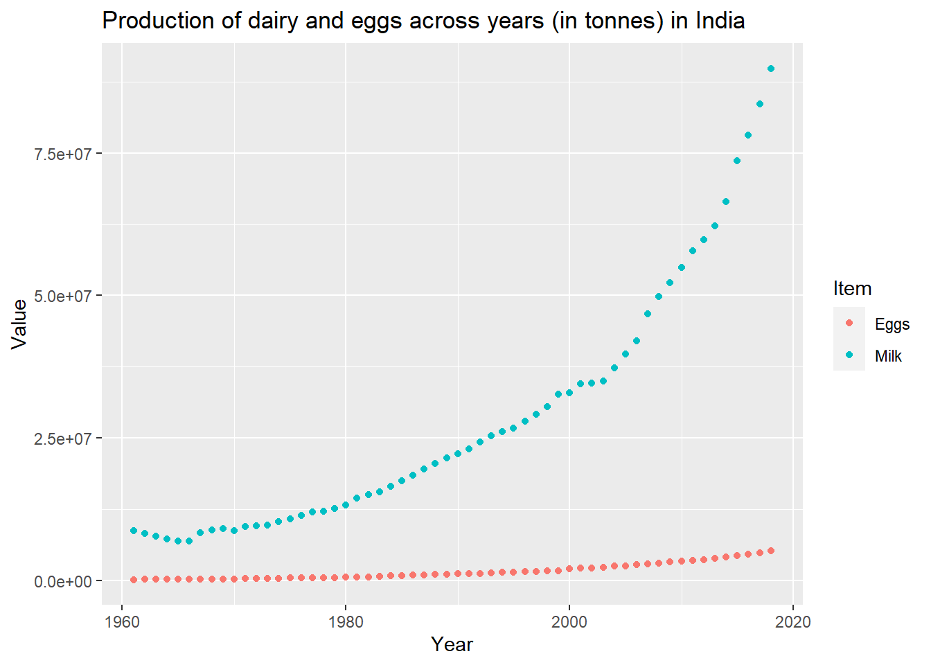
Before analysis, I filtered the dataset to only have the production values since these were measured by the same quantity(tonnes) for milk and eggs. Hence they could be compared. Moreover, I filtered the data to have values from India.
In the scatterplot below, it is evident that the milk production has increased at a rapid rate from 1961 to 2018. This could correspond to the increase in population and popular consumption of milk. However, the eggs production has not had such a rapid increase in the same time period. This may be attributed to the fact that several Indians follow a vegetarian diet which does not include the consumption of eggs.

new_dairy_egg_sub<-new_dairy_egg%>%filter(Element=="Production")%>%filter(Area=="India")
#year,item,value

ggplot(new_dairy_egg_sub, aes(x=Year,y=Value, color=Item)) +
     geom_point() +
     labs(title = "Production of dairy and eggs across years (in tonnes) in India")